Pyflex

Pyflex is a Python port of the FLEXWIN algorithm for automatically selecting windows for seismic tomography. For the most part it mimicks the calculations of the original FLEXWIN package; minor differences and their reasoning are detailed later.

To give credit where credit is due, the original FLEXWIN program can be downloaded here, the corresponding publication is

Maggi, A., Tape, C., Chen, M., Chao, D., & Tromp, J. (2009). An automated time-window selection algorithm for seismic tomography. Geophysical Journal International, 178(1), 257–281 doi:10.1111/j.1365-246X.2009.04099.x

If you use Pyflex, please also cite the latest released version: http://dx.doi.org/10.5281/zenodo.31607

The source code for Pyflex lives on Github: https://github.com/krischer/pyflex. If you encounter any problems with it please open an issue or submit a pull request.

Installation

Pyflex utilizes ObsPy (and some of its dependencies) for the processing and data handling. As a first step, please follow the installation instructions of ObsPy for your given platform (we recommend the installation with Anaconda as it will most likely result in the least amount of problems). Pyflex should work with Python versions 2.7, 3.3, and 3.4 (mainly depends on the used ObsPy version). To install it, best use pip:

$ pip install pyflex

If you want the latest development version, or want to work on the code, you will have to install with the help of git.

$ git clone https://github.com/krischer/pyflex.git
$ cd pyflex
$ pip install -v -e .

Tests

To assure the installation is valid and everything works as expected, run the tests with

$ python -m pyflex.tests

Usage

The first step is to import ObsPy and Pyflex.

%pylab inline
import obspy
import pyflex

Populating the interactive namespace from numpy and matplotlib

Pyflex expects both observed and synthetic data to already be fully processed. An easy way to accomplish this is to utilize ObsPy. This example reproduces what the original FLEXWIN package does when it is told to also perform the filtering.

obs_data = obspy.read("../src/pyflex/tests/data/1995.122.05.32.16.0000.II.ABKT.00.LHZ.D.SAC")
synth_data = obspy.read("../src/pyflex/tests/data/ABKT.II.LHZ.semd.sac")

obs_data.detrend("linear")
obs_data.taper(max_percentage=0.05, type="hann")
obs_data.filter("bandpass", freqmin=1.0 / 150.0, freqmax=1.0 / 50.0,
                corners=4, zerophase=True)

synth_data.detrend("linear")
synth_data.taper(max_percentage=0.05, type="hann")
synth_data.filter("bandpass", freqmin=1.0 / 150.0, freqmax=1.0 / 50.0,
                  corners=4, zerophase=True)

1 Trace(s) in Stream:
II.ABKT..LHZ | 1995-05-02T05:57:53.500006Z - 1995-05-02T08:06:13.500006Z | 1.0 Hz, 7701 samples

The configuration is encapsuled within a Config object. It thus replaces the need for a PAR_FILE and the user functions. Please refer to the Config object’s documentation for more details.

config = pyflex.Config(
    min_period=50.0, max_period=150.0,
    stalta_waterlevel=0.08, tshift_acceptance_level=15.0,
    dlna_acceptance_level=1.0, cc_acceptance_level=0.80,
    c_0=0.7, c_1=4.0, c_2=0.0, c_3a=1.0, c_3b=2.0, c_4a=3.0, c_4b=10.0)

Observed and synthetic waveforms can be passed as either ObsPy Trace objects, or Stream objects with one component. The optional plot parameter determines if a plot is produced or not. The select_windows() function is the high level interface suitable for most users of Pyflex. Please refer to its documentation for further details.

windows = pyflex.select_windows(obs_data, synth_data, config, plot=True)

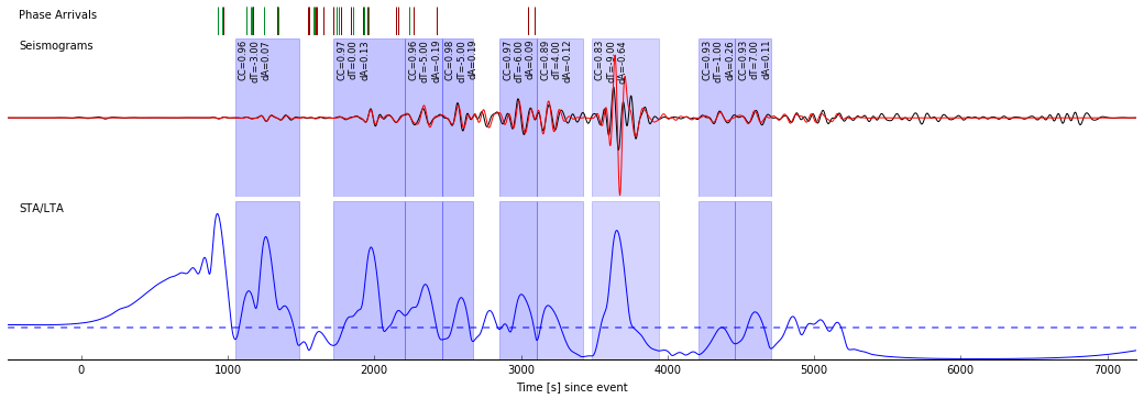
Windows

It returns a sorted list of Window objects which can then be used in further applications.

import pprint
pprint.pprint(windows[:3])

[Window(left=1551, right=1985, center=1768, channel_id=II.ABKT.00.LHZ, max_cc_value=0.957407008229, cc_shift=-3, dlnA=0.0746904099861),
 Window(left=2221, right=2709, center=2465, channel_id=II.ABKT.00.LHZ, max_cc_value=0.966468650943, cc_shift=0, dlnA=0.128083046189),
 Window(left=2709, right=2960, center=2834, channel_id=II.ABKT.00.LHZ, max_cc_value=0.963357158929, cc_shift=-5, dlnA=-0.192769044168)]

Each window contains a number of properties that can be used to calculate absolute and relative times for the specific window. left and right specify the boundary indices of a window, absolute_starttime and absolute_endtime are the absolute times of a window’s bounds as ObsPy UTCDateTime objects, and relative_starttime and relative_endtime are the bounds of a window in seconds since the first sample of the data arrays (not necessarily identical to the event origin time!).

win = windows[4]
print("Indices: %s - %s" % (win.left, win.right))
print("Absolute times: %s - %s" % (win.absolute_starttime, win.absolute_endtime))
print("Relative times in seconds: %s - %s" % (win.relative_starttime,
                                              win.relative_endtime))

Indices: 3353 - 3609
Absolute times: 1995-05-02T06:53:46.500006Z - 1995-05-02T06:58:02.500006Z
Relative times in seconds: 3353.0 - 3609.0

A window furthermore contains a list of phases theoretically arriving within the window. Take care that the times here are in seconds since the event origin.

win.phase_arrivals

[{u'name': u'SKSSKS', u'time': 3049.8839177900104},
 {u'name': u'SKIKSSKIKS', u'time': 3091.6546087871261}]

Event and Station Information

While Pyflex can also operate without any event and station information, it needs some information to work at full efficiency. In case the waveform traces originate from SAC files, they might contain the necessary information. Pyflex is able to extract that information but this should really be seen as a last resort.

The easiest way to pass the necessary information to Pyflex is to use its very bare bones event and station objects.

event = pyflex.Event(latitude=-3.77, longitude=-77.07, depth_in_m=112800,
                     origin_time=obspy.UTCDateTime(1995, 5, 2, 6, 6, 13))
station = pyflex.Station(latitude=37.93, longitude=58.12)

windows = pyflex.select_windows(obs_data, synth_data, config,
                                event=event, station=station)

A more powerful approach enabling the construction of cleaner workflows is to pass ObsPy objects. Event information can be passed as ObsPy Catalog or Event objects. Station information on the other hand can be passed as an Inventory object. This enables the acquisition of this information directly from web services or QuakeML/StationXML files on dics. Please refer to the ObsPy documentation for more details.

event = obspy.readEvents("../events/event_1.xml")
station = obspy.read_inventory("../stations/II_ABKT.xml")
windows = pyflex.select_windows(obs_data, synth_data, config,
                                event=event, station=station)

(De)Serializing Windows

In case necessary, windows can also be written to and read from disc. Pyflex utilizes a simple JSON representation of the windows. The windows_filename parameter determines the filename if given.

windows = pyflex.select_windows(obs_data, synth_data, config,
                                windows_filename="windows.json")

The resulting JSON file will have a list of Window objects under the "windows" key.

{
    "windows": [
        {
            "absolute_endtime": "1995-05-02T06:30:58.500006Z",
            "absolute_starttime": "1995-05-02T06:23:44.500006Z",
            "cc_shift_in_samples": -3,
            "cc_shift_in_seconds": -3.0,
            "center_index": 1768,
            "channel_id": "II.ABKT.00.LHZ",
            "dlnA": 0.07469040998606906,
            "dt": 1.0,
            "left_index": 1551,
            "max_cc_value": 0.957407008228736,
            "min_period": 50.0,
            "phase_arrivals": [
                {
                    "name": "PKIKP",
                    "time": 1130.1899293364668
                },
                {

To read the windows again you will have to utilize the lower level WindowSelector class. There is no higher level interface for this as it is likely an edge use case. The window criteria like cross correlation and amplitude misfit will be recalculated upon loading to assure consistency with the data.

ws2 = pyflex.WindowSelector(obs_data, synth_data, config)
print("Windows before loading: %i" % len(ws2.windows))
ws2.load("windows.json")
print("Windows after loading: %i" % len(ws2.windows))

Windows before loading: 0
Windows after loading: 9

Difference to the original FLEXWIN algorithm

Pyflex largely follows the original FLEXWIN algorithm. The major differences are outlined here.

• The found local extrema of the STA/LTA functional might differ a bit. In case of a “flat” extrema, Pyflex will always find the leftmost index.
• The order of rejection stages has been changed a bit to assure cheaper eliminations are run first. This results in a significant speed boost.
• The water/acceptance level of the data fit criteria is now evaluated at the center of each windows and not at the central peak.
• The Config object has a min_surface_wave_velocity parameter which can be used to easily discard windows for late arriving surface/coda waves.

Overlap Resolution Strategy

Instead of using the overlap resolution strategy outlined in section 2.5 Stage E in the FLEXWIN paper, Pyflex utilizes weighted interval scheduling which is a classical IT problem. The weighted interval scheduling algorithm finds the best possible subset of non-overlapping windows by maximizing the cumulative weight of all chosen windows. By default the weight of each window is its length in terms of minimum period of the data times the maximum cross correlation coefficient. The weighting function can be overwritten with the help of the Config object. This results in similar windows to the original FLEXWIN algorithm but is easier to reason about.

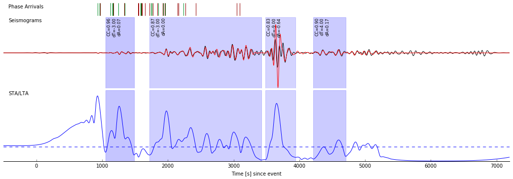
Pyflex furthermore offers the option to merge all good candidate windows. This is useful for some misfit measurements.

config = pyflex.Config(
    min_period=50.0, max_period=150.0,
    stalta_waterlevel=0.08, tshift_acceptance_level=15.0,
    dlna_acceptance_level=1.0, cc_acceptance_level=0.80,
    c_0=0.7, c_1=4.0, c_2=0.0, c_3a=1.0, c_3b=2.0, c_4a=3.0, c_4b=10.0,
    resolution_strategy="merge")
windows = pyflex.select_windows(obs_data, synth_data, config, plot=True)

Logging

By default, Pyflex is fairly quiet and will only raise exceptions and warnings in case they occur. Pyflex utilizes Python’s logging facilities so if you want more information you can hook into them. This approach is very flexible as it allows you to install custom logging handlers and channels.

import logging
logger = logging.getLogger("pyflex")
logger.setLevel(logging.DEBUG)

windows = pyflex.select_windows(obs_data, synth_data, config)

[2017-07-11 13:23:44,651] - pyflex - INFO: Extracted station information from observed SAC file.
[2017-07-11 13:23:44,652] - pyflex - INFO: Extracted event information from observed SAC file.
[2017-07-11 13:23:45,196] - pyflex - INFO: Calculated travel times.
[2017-07-11 13:23:45,198] - pyflex - INFO: Calculating envelope of synthetics.
[2017-07-11 13:23:45,200] - pyflex - INFO: Calculating STA/LTA.
[2017-07-11 13:23:45,241] - pyflex - INFO: Initial window selection yielded 1663 possible windows.
[2017-07-11 13:23:45,251] - pyflex - INFO: Rejection based on travel times retained 1663 windows.
[2017-07-11 13:23:45,266] - pyflex - INFO: Rejection based on minimum window length retained 1653 windows.
[2017-07-11 13:23:45,336] - pyflex - INFO: Water level rejection retained 36 windows
[2017-07-11 13:23:45,340] - pyflex - INFO: Single phase group rejection retained 14 windows
[2017-07-11 13:23:45,341] - pyflex - INFO: Removing duplicates retains 14 windows.
[2017-07-11 13:23:45,342] - pyflex - INFO: Rejection based on minimum window length retained 14 windows.
[2017-07-11 13:23:45,343] - pyflex - INFO: SN amplitude ratio window rejection retained 14 windows
[2017-07-11 13:23:45,346] - pyflex - INFO: Rejection based on data fit criteria retained 14 windows.
[2017-07-11 13:23:45,349] - pyflex - INFO: Merging windows resulted in 4 windows.

API Documentation

This section documents the most used functions and classes. For more details you can always have a look at the code.

Config Object

class pyflex.config.Config(min_period, max_period, stalta_waterlevel=0.07, tshift_acceptance_level=10.0, tshift_reference=0.0, dlna_acceptance_level=1.3, dlna_reference=0.0, cc_acceptance_level=0.7, s2n_limit=1.5, earth_model=u’ak135’, min_surface_wave_velocity=3.0, max_time_before_first_arrival=50.0, c_0=1.0, c_1=1.5, c_2=0.0, c_3a=4.0, c_3b=2.5, c_4a=2.0, c_4b=6.0, check_global_data_quality=False, snr_integrate_base=3.5, snr_max_base=3.0, noise_start_index=0, noise_end_index=None, signal_start_index=None, signal_end_index=-1, window_weight_fct=None, window_signal_to_noise_type=u’amplitude’, resolution_strategy=u’interval_scheduling’)

Central configuration object for Pyflex.

This replaces the old PAR_FILEs and user functions. It has sensible defaults for most values but you will probably want to adjust them for your given application.

If necessary, the acceptance levels/limits can also be set as arrays. Each array must have the same number of samples as the observed and synthetic data. The corresponding values are then evaluated seperately at each necessary point. This enables the full emulation of the user functions in the original FLEXWIN code. The following basic example illustrates the concept which can become arbitrarily complex.

stalta_waterlevel = 0.08 * np.ones(npts)
tshift_acceptance_level = 15.0 * np.ones(npts)
dlna_acceptance_level = 1.0 * np.ones(npts)
cc_acceptance_level = 0.80 * np.ones(npts)
s2n_limit = 1.5 * np.ones(npts)

# Double all values from a certain index on.
stalta_waterlevel[2500:] *= 2.0
tshift_acceptance_level[2500:] += 5.0
dlna_acceptance_level[2500:] *= 1.5
cc_acceptance_level[2500:] += 0.5
s2n_limit[2500:] *= 0.9

config = Config(
    min_period=10.0, max_period=50.0,
    stalta_waterlevel=stalta_waterlevel,
    tshift_acceptance_level=tshift_acceptance_level,
    dlna_acceptance_level=dlna_acceptance_level,
    cc_acceptance_level=cc_acceptance_level,
    s2n_limit=s2n_limit)

Parameters:

• min_period (float) – Minimum period of the filtered input data in seconds.
• max_period (float) – Maximum period of the filtered input data in seconds.
• stalta_waterlevel (float or numpy.ndarray) – Water level on the STA/LTA functional. Can be either a single value or an array with the same number of samples as the data.
• tshift_acceptance_level (float or numpy.ndarray) – Maximum allowable cross correlation time shift/lag relative to the reference. Can be either a single value or an array with the same number of samples as the data.
• tshift_reference (float) – Allows a systematic shift of the cross correlation time lag.
• dlna_acceptance_level (float or numpy.ndarray) – Maximum allowable amplitude ratio relative to the reference. Can be either a single value or an array with the same number of samples as the data.
• dlna_reference (float) – Reference DLNA level. Allows a systematic shift.
• cc_acceptance_level (float or numpy.ndarray) – Limit on the normalized cross correlation per window. Can be either a single value or an array with the same number of samples as the data.
• s2n_limit (float or numpy.ndarray) – Limit of the signal to noise ratio per window. If the maximum amplitude of the window over the maximum amplitude of the global noise of the waveforms is smaller than this window, then it will be rejected. Can be either a single value or an array with the same number of samples as the data.
• earth_model (str) – The earth model used for the traveltime calculations. Either "ak135" or "iasp91".
• min_surface_wave_velocity (float) – The minimum surface wave velocity in km/s. All windows containing data later then this velocity will be rejected. Only used if station and event information is available.
• max_time_before_first_arrival (float) – This is the minimum starttime of any window in seconds before the first arrival. No windows will have a starttime smaller than this.
• c_0 (float) – Fine tuning constant for the rejection of windows based on the height of internal minima. Any windows with internal minima lower then this value times the STA/LTA water level at the window peak will be rejected.
• c_1 (float) – Fine tuning constant for the minimum acceptable window length. This value multiplied by the minimum period will be the minimum acceptable window length.
• c_2 (float) – Fine tuning constant for the maxima prominence rejection. Any windows whose minima surrounding the central peak are smaller then this value times the central peak will be rejected. This value is set to 0 in many cases as it is hard to control.
• c_3a (float) – Fine tuning constant for the separation height in the phase separation rejection stage.
• c_3b (float) – Fine tuning constant for the separation time used in the decay function in the phase separation rejection stage.
• c_4a (float) – Fine tuning constant for curtailing windows on the left with emergent start/stops and/or codas.
• c_4b (float) – Fine tuning constant for curtailing windows on the right with emergent start/stops and/or codas.
• check_global_data_quality – Determines whether or not to check the signal to noise ratio of the whole observed waveform. If True, no windows will be selected if the signal to noise ratio is above the thresholds.
• snr_integrate_base (float) – Minimal SNR ratio. If the squared sum of the signal normalized by its length over the squared sum of the noise normalized by its length is smaller then this value, no windows will be chosen for the waveforms. Only used if check_global_data_quality is True.
• snr_max_base (float) – Minimal amplitude SNR ratio. If the maximum amplitude of the signal over the maximum amplitude of the noise is smaller than this value no windows will be chosen for the waveforms. Only used if check_global_data_quality is True.
• noise_start_index (int) – Index in the observed data where noise starts for the signal to noise calculations.
• noise_end_index (int) – Index in the observed data where noise ends for the signal to noise calculations. Will be set to the time of the first theoretical arrival minus the minimum period if not set and event and station information is available.
• signal_start_index (int) – Index where the signal starts for the signal to noise calculations. Will be set to to the noise end index if not given.
• signal_end_index (int) – Index where the signal ends for the signal to noise calculations.
• window_weight_fct (function) – A function returning the weight for a specific window as a single number. Directly passed to the Window ‘s initialization function.
• window_signal_to_noise_type (str) – The type of signal to noise ratio used to reject windows. If "amplitude", then the largest amplitude before the arrival is the noise amplitude and the largest amplitude in the window is the signal amplitude. If "energy" the time normalized energy is used in both cases. The later one is a bit more stable when having random wiggles before the first arrival.
• resolution_strategy (str) – Strategy used to resolve overlaps. Possibilities are "interval_scheduling" and "merge". Interval scheduling will chose the optimal subset of non-overlapping windows. Merging will simply merge overlapping windows.

Main select_windows() function

pyflex.flexwin.select_windows(observed, synthetic, config, event=None, station=None, plot=False, plot_filename=None, windows_filename=None)

Convenience function for selecting (and plotting) windows.

Parameters:

• observed (Trace or single component Stream) – The preprocessed, observed waveform.
• observed – The preprocessed, synthetic waveform.
• config (Config) – Configuration object.
• event (A Pyflex Event object, an ObsPy Catalog object, or an ObsPy Event object) – The event information. Either a Pyflex Event object, or an ObsPy Catalog or Event object. If not given this information will be extracted from the data traces if either originates from a SAC file.
• station (A Pyflex Station object or an ObsPy Inventory object) – The station information. Either a Pyflex Station object, or an ObsPy Inventory. If not given this information will be extracted from the data traces if either originates from a SAC file.
• plot (bool) – Plot the resulting windows.
• plot_filename (str) – If plot is True, this gives the possibility to specify a filename for the plot. The fileformat will be determines from that name. If not given, the plot will be shown with pylab’s show() function.
• windows_filename (str or file-like object.) – If given, windows will be saved to that file or file-like object. Pyflex utilizes a custom JSON format for that.

The Window Object

Pyflex internally utilizes a window class for candidates and final windows, the select_windows() function will return a list of these.

class pyflex.window.Window(left, right, center, time_of_first_sample, dt, min_period, channel_id, weight_function=None)

Class representing window candidates and final windows.

The optional weight_function parameter can be used to customize the weight of the window. Its single parameter is an instance of the window. The following example will create a window function that does exactly the same as the default weighting function.

>>> def weight_function(win):
...     return ((win.right - win.left) * win.dt / win.min_period *
...         win.max_cc_value)

Parameters:

• left (int) – The array index of the left bound of the window.
• right (int) – The array index of the right bound of the window.
• center (int) – The array index of the central maximum of the window.
• time_of_first_sample (UTCDateTime) – The absolute time of the first sample in the array. Needed for the absolute time calculations.
• dt (float) – The sample interval in seconds.
• min_period (float) – The minimum period in seconds.
• channel_id (str) – The id of the channel of interest. Needed for a useful serialization.
• weight_function (function) – Function determining the window weight. The only argument of the function is a window instance.

absolute_endtime

Absolute time of the right border of this window.

absolute_starttime

Absolute time of the left border of this window.

relative_endtime

Relative time of the right border in seconds to the first sample in the array.

relative_starttime

Relative time of the left border in seconds to the first sample in the array.

weight

The weight of the window used for the weighted interval scheduling. Either calls a potentially passed window weight function or defaults to the window length in number of minimum periods times the cross correlation coefficient.

Helper Objects

These are simple helper objects giving the capability of specifying event and station information without having to resort to full blown ObsPy objects (altough this is also supported and likely results in a cleaner workflow).

class pyflex.Event(latitude, longitude, depth_in_m, origin_time)

Create new instance of Event(latitude, longitude, depth_in_m, origin_time)

class pyflex.Station(latitude, longitude)

Create new instance of Station(latitude, longitude)

Exceptions and Warnings

Right now error handling is very simple and handled by these two types.

class pyflex.PyflexError

Base class for all Pyflex exceptions. Will probably be used for all exceptions to not overcomplicate things as the whole package is pretty small.

class pyflex.PyflexWarning

Base class for all Pyflex warnings.

Low-level WindowSelector Class

For most purposes, the select_windows() function it the better choice, but this might be useful in some more advanced cases.

class pyflex.window_selector.WindowSelector(observed, synthetic, config, event=None, station=None)

Low level window selector internally used by Pyflex.

Parameters:

• observed (Trace or single component Stream) – The preprocessed, observed waveform.
• synthetic (Trace or single component Stream) – The preprocessed, synthetic waveform.
• config (Config) – Configuration object.
• event (A Pyflex Event object, an ObsPy Catalog object, or an ObsPy Event object) – The event information. Either a Pyflex Event object, or an ObsPy Catalog or Event object. If not given this information will be extracted from the data traces if either originates from a SAC file.
• station (A Pyflex Station object or an ObsPy Inventory object) – The station information. Either a Pyflex Station object, or an ObsPy Inventory. If not given this information will be extracted from the data traces if either originates from a SAC file.

attach_phase_arrivals_to_windows()

Attaches the theoretical phase arrivals to the windows.

calculate_preliminiaries()

Calculates the envelope, STA/LTA and the finds the local extrema.

calculate_ttimes()

Calculate theoretical travel times. Only call if station and event information is available!

check_data_quality()

Checks the data quality by estimating signal to noise ratios.

curtail_length_of_windows()

Curtail the window length. Equivalent to a call to curtail_window_length() in the original flexwin code.

determine_signal_and_noise_indices()

Calculate the time range of the noise and the signal respectively if not yet specified by the user.

initial_window_selection()

Find all possible windows. This is equivalent to the setup_M_L_R() function in flexwin.

load(filename)

Load windows from a JSON file and attach them to the current window selector object.

Parameters:filename (str or file-like object) – The filename or file-like object to load.

merge_windows()

Merge overlapping windows. Will also recalculate the data fit criteria.

minimum_window_length

Minimum acceptable window length.

plot(filename=None)

Plot the current state of the windows.

Parameters:filename (str) – If given, the plot will be written to this file, otherwise the plot will be shown.

reject_based_on_data_fit_criteria()

Rejects windows based on similarity between data and synthetics.

reject_based_on_signal_to_noise_ratio()

Rejects windows based on their signal to noise amplitude ratio.

reject_on_minima_water_level()

Filter function rejecting windows whose internal minima are below the water level of the windows peak. This is equivalent to the reject_on_water_level() function in flexwin.

reject_on_phase_separation()

Reject windows based on phase seperation. Equivalent to reject_on_phase_separation() in the original flexwin code.

reject_on_prominence_of_central_peak()

Equivalent to reject_on_prominence() in the original flexwin code.

reject_on_traveltimes()

Reject based on traveltimes. Will reject windows containing only data before a minimum period before the first arrival and windows only containing data after the minimum allowed surface wave speed. Only call if station and event information is available!

reject_windows_based_on_minimum_length()

Reject windows smaller than the minimal window length.

remove_duplicates()

Filter to remove duplicate windows based on left and right bounds.

This function will also change the middle to actually be in the center of the window. This should result in better results for the following stages as lots of thresholds are evaluated at the center of a window.

schedule_weighted_intervals()

Run the weighted interval scheduling.

select_windows()

Launch the window selection.

write(filename)

Write windows to the specified filename or file like object.

Will be written as a custom JSON file.

Parameters:filename (str or file-like object) – Name or object to write to.

Misc Functionality

pyflex.interval_scheduling.schedule_weighted_intervals(I)

Use dynamic algorithm to schedule weighted intervals

sorting is O(n log n), finding p[1..n] is O(n log n), finding OPT[1..n] is O(n), selecting is O(n) whole operation is dominated by O(n log n)

pyflex.utils.find_local_extrema(data)

Function finding local extrema. It can also deal with flat extrema, e.g. a flat top or bottom. In that case the first index of all flat values will be returned.

Returns a tuple of maxima and minima indices.

pyflex.stalta.sta_lta(data, dt, min_period)

STA/LTA as used in FLEXWIN.

Parameters:

• data – The data array.
• dt – The sample interval of the data.
• min_period – The minimum period of the data.